Cloud Radar System (CRS) Reflectivity and Doppler Velocity Quick View
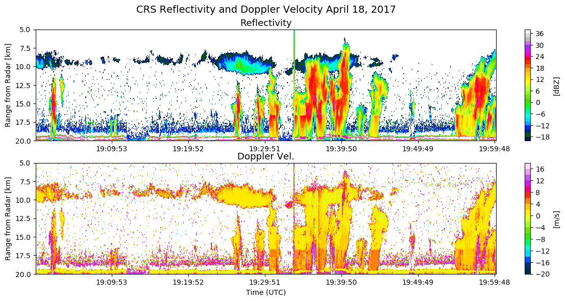
The Cloud Radar System (CRS) is a 94 GHz, W-band polarimetric Doppler radar built to operate onboard the NASA ER-2 high-altitude research aircraft. CRS was used to capture high-resolution profiles of reflectivity and Doppler velocity from an altitude of approximately 20 km. This data recipe enables users to generate time-height plots of the measured CRS radar reflectivity and Doppler velocity through a Python 3 plotting routine.
| Data Recipe Type | |
|---|---|
 | |
| Data Visualization | |
| TYPE | ACCESS | ||
|---|---|---|---|
|
| Python Script (Main) |
| Open Source |
|
| Python Script (Functions) |
| Open Source |
This data recipe was developed for the most recent Cloud Radar System (CRS) dataset holdings at the NASA Global Hydrometeorology Resource Center (GHRC) Distributed Active Archive Center (DAAC). These datasets include the Cloud Radar System (CRS) IMPACTS dataset in HDF-5 format, GOES-R PLT Cloud Radar System (CRS) dataset in netCDF-3 format, the GPM Ground Validation Cloud Radar System (CRS) OLYMPEX dataset in netCDF-3 format, and the GPM Ground Validation Cloud Radar System (CRS) IPHEx dataset in netCDF-3 format. This data recipe does not provide plotting capabilities for the TCSP Cloud Radar System (CRS) dataset in ASCII format, however, browse images of the plotted TCSP CRS reflectivity and Doppler velocity data are available here.
This data recipe is available as two Python 3 scripts: one containing the main code and the other containing the functions used in the main code. To run the scripts, please install the following Python packages: numpy, xarray, netCDF4, h5py, and matplotlib. Additional information on installing Python packages is available here.
Follow this link to the GHRC DAAC Data-Recipes GitHub folder and obtain the Python scripts named “CRS_Recipe_Code.ipynb” and “CRS_Recipe_Functions.ipynb”. The “CRS_Recipe_Code.ipynb” script contains the main code that will read the CRS data files. The “CRS_Recipe_Functions.ipynb” script contains the functions that will be used in the primary “CRS_Recipe_Code.ipynb” script.
You can preview the scripts by clicking the file name. To download the scripts, go to the GHRC DAAC Data-Recipes GitHub folder, click the green “Code” button located in the top right corner of the display window, and choose "Download ZIP". Save the zip file to a desired location on your computer and unzipp it to get all GHRC data recipe codes including “CRS_Recipe_Code.ipynb” and “CRS_Recipe_Functions.ipynb”. They are JSON IPython notebook documents (.ipynb) created by Jupyter Notebook. One can easily convert a ipynb notebook file to regular python script (.py) via command line below:
$ ipython nbconvert --to=python [YOUR_NOTEBOOK].ipynb
To download the data needed for this data recipe, a free NASA Earthdata user account is required. If you do not have an account, you will first need to create one by clicking the “Register” button (shown below) and following the required steps.
Once your NASA Earthdata account has been created, you can now download CRS data files (you may have to re-enter your Earthdata account information if you are not already logged in).
You can download the CRS dataset files from each field campaign dataset landing page accessed through the GHRC Search Portal. These landing pages can be found by searching the term "CRS" or selecting "CRS" from the "Instrument" drop down menu for search filters. Clicking one of the CRS dataset links listed from the search will bring you to that dataset’s landing page (Note: links to these landing pages are also included in the “How to Use” section above). Here, you can click the “File list” button to view a list of the files available for that particular dataset. To download a file individually, click a file link and the file will be downloaded to your computer. To bulk download CRS data files, you can click the “Download Data” button on the dataset landing page. A tutorial on how to bulk download data files from HyDRO 2.0 can be found on the GHRC Search Portal Help Page. The NASA Earthdata Search platform can also be used to download CRS data. Search the term "CRS" followed by the desired field campaign dataset acronym (e.g. IMPACTS, GOES-R PLT, OLYMPEX or IPHEx) in the Earthdata Search search box to locate the CRS dataset of choice. Save the files to a desired location on your computer.
There are two ways to run the CRS Python script: from your computer’s command prompt or from your Python console. To run the script from the command prompt, first open your computer’s prompt window and check that your current directory is the location where the “CRS_Recipe_Code.py” and “CRS_Recipe_Functions.py” scripts are saved. Make sure the required Python packages outlined in the “How to Use” section are installed. The following arguments will be passed in the command line. After initiating Python by typing “python”, add a space and paste the name of the script: “CRS_Recipe_Code.py”. Add a space and then enter the path to the directory holding the CRS files you downloaded and press “Enter” on your keyboard. An example of the command line statement is shown below:
Windows
C:\Users\name> python CRS_Recipe_Code.py C:\Users\name\data_recipes\crs\
Linux
$ python CRS_Recipe_Code.py /home/user/data_recipes/crs/
The code will lead you through a series of prompts to select the dataset you would like to plot, which flight period you would like to plot, whether you would like to plot a subset or the entire flight period, and whether you would like to save the plot image. If you would like to change the directory from which the CRS data files are selected and plotted, enter the “Q” option (quit) to exit the code and then re-run the script with the same format shown in the example above except with the new directory path. An example of the plotting procedure on Windows is shown in the following steps to generate the image seen at the beginning of this data recipe.
Note: The CRS data files are available for a variety of flight periods. Some files contain long periods of flight data that can use large amounts of memory on your computer when trying to plot the data using this data recipe. If the code produces a memory error, try plotting a smaller subset time period that can be managed by your computer’s memory system.
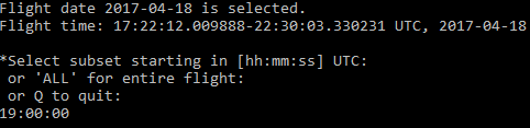
When the script is first run, the code will ask you which CRS campaign dataset you would like to plot. In this example we will plot data from the GOES-R PLT field campaign, therefore we entered “2” for the campaign number.

It will then ask which flight period you would like to plot. There was only one GOES-R PLT data file in the directory for this example, therefore there is one option for GOES-R PLT flight dates. The flight date “April 18, 2017” was selected.

Next, the code will give you the option to plot a subset or the entire flight period. For this example we will plot a subset. When plotting a subset, the code asks for the desired subset starting time. For the plot displayed in this tutorial, this time will be “19:00:00” UTC. (Note: For the IMPACTS dataset plotting routine, the code will ask the user to enter the starting date after asking for the starting time.)
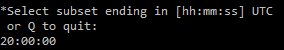
The code will then ask for the desired subset ending time. For the plot displayed at the beginning of this tutorial, the subset ending time will be “20:00:00” UTC. (Note: For the IMPACTS dataset plotting routine, the code will ask the user to enter the ending date after asking for the ending time.)
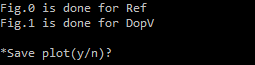
The code will notify you when the plot figures have been generated for "reflectivity" and "Doppler velocity". The plot will display in the matplotlib figure window (Windows only) where it can be viewed. Once you close the plot display window, the code will ask whether you would like to save the plot.
Open the Python environment installed on your computer and as previously noted, make sure the required Python packages outlined in the “How to Use” section are installed.
Navigate to the location on your computer where the “CRS_Recipe_Code.py” and “CRS_Recipe_Functions.py” files are saved and open the “CRS_Recipe_Code.py” file within your Python environment.
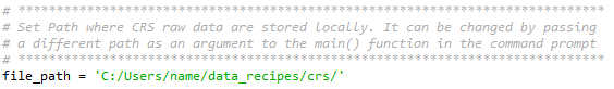
At the very beginning of the “CRS_Recipe_Code.py” script is a header that describes the script’s function. Below the header, all of the required packages and subpackages are imported. Using your computer’s file explorer, navigate to the folder on your computer where you saved the CRS data files. From the address bar, copy the file path and paste it inside the quotations behind the “dirpath” variable. Change all of the backslashes (\) to forward slashes (/) in the path name. An example path is included in the script and shown in the image below.
When the “CRS_Recipe_Code.py” script is run, it will ask the user to input which CRS campaign dataset they would like to plot, the flight date and period they would like to plot, the subset time period of their choosing (or “ALL” for the entire flight), and whether they would like to save the generated PNG plot image.
After running the script from either your computer’s command prompt or your Python console and entering the information requested by each prompt, the final plot will display like the image below. Detailed documentation of each portion of the code is included inside the “CRS_Recipe_Code.py” and “CRS_Recipe_Functions.py” scripts.

| Dataset Name | Cloud Radar System (CRS) IMPACTS |
| Platform | NASA Earth Resources 2 (ER-2) high-altitude aircraft |
| Instrument | Cloud Radar System (CRS) |
| Science Parameter | Radar reflectivity and Doppler velocity |
| Format | HDF5 |
| Data Information |
|
| Dataset Name | GOES-R PLT Cloud Radar System (CRS) |
| Platform | NASA Earth Resources 2 (ER-2) high-altitude aircraft |
| Instrument | Cloud Radar System (CRS) |
| Science Parameter | Radar reflectivity and Doppler velocity |
| Format | netCDF-3 |
| Data Information |
|
| Dataset Name | GPM Ground Validation Cloud Radar System (CRS) OLYMPEX |
| Platform | NASA Earth Resources 2 (ER-2) high-altitude aircraft |
| Instrument | Cloud Radar System (CRS) |
| Science Parameter | Radar reflectivity and Doppler velocity |
| Format | netCDF-3 |
| Data Information |
|
| Dataset Name | GPM Ground Validation Cloud Radar System (CRS) IPHEx |
| Platform | NASA Earth Resources 2 (ER-2) high-altitude aircraft |
| Instrument | Cloud Radar System (CRS) |
| Science Parameter | Radar reflectivity and Doppler velocity |
| Format | netCDF-3 |
| Data Information |
|
| Variable | Description | Dimension | Units |
|---|---|---|---|
| dBZe | Radar Reflectivity | Time, range | dBZ |
| Velocity | Doppler Velocity | Time, range | m/s |
| Variable | Description | Dimension | Units |
|---|---|---|---|
| ref | Radar Reflectivity | Time, range | dBZ |
| dop | Doppler Velocity after corrected for aircraft motion and folding | Time, range | m/s |
| Variable | Description | Dimension | Units |
|---|---|---|---|
| zku | Radar Reflectivity | Time, range | dBZ |
| dopcorr | Doppler Velocity after corrected for aircraft motion and folding | Time, range | m/s |
| Variable | Description | Dimension | Units |
|---|---|---|---|
| zku | Radar Reflectivity | Time, range | dBZ |
| dopcorr | Doppler Velocity after corrected for aircraft motion and folding | Time, range | m/s |

Jan 9th, 2023