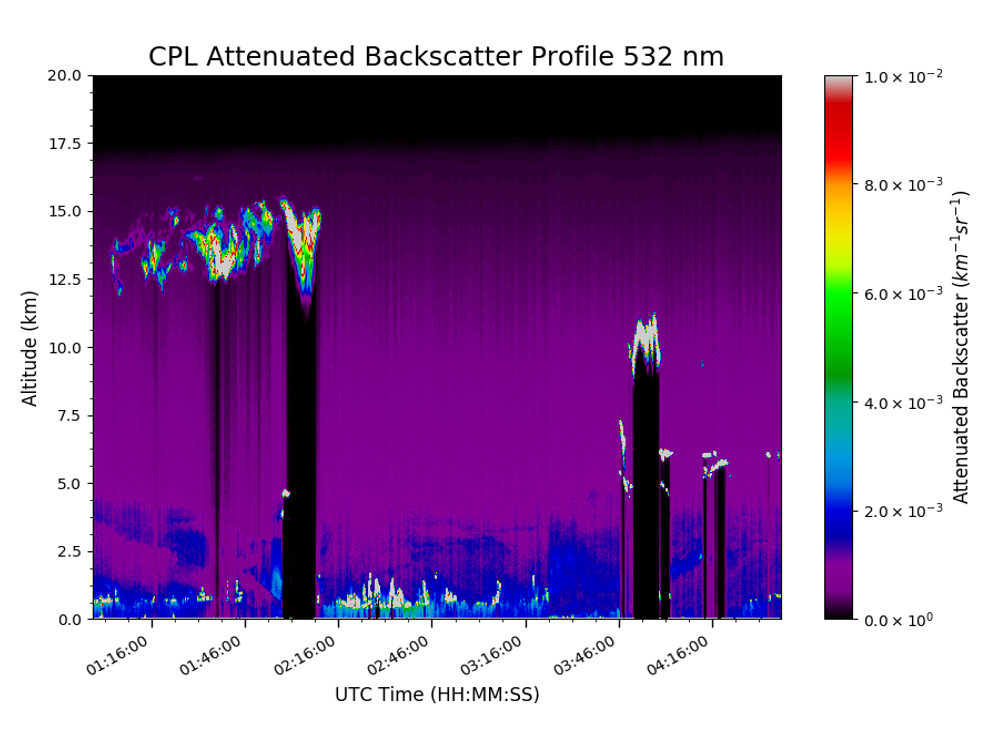
HS3 CPL Attenuated Total Backscatter Quickview
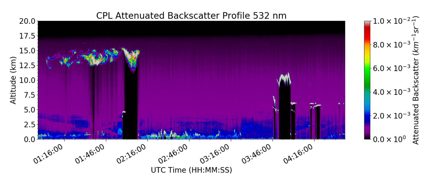
The Hurricane and Severe Storm Sentinel (HS3) airborne field campaign used the Cloud Precipitation Lidar (CPL) instrument to collect measurements of cloud, precipitation, and aerosol features of tropical cyclones. This data recipe instructs users on how to generate vertical time-height plots of HS3 CPL attenuated total backscatter measurements using a Python plotting routine. The Python routine requires users to define the GHRC OPeNDAP path to a datafile and the spectral channel the measurements were collected. To run this Python routine, a pre-installed version of Python and additional Python packages are required. Advanced users may alter the code to plot other data variables.
| Data Recipe Type | |
|---|---|
| Visualization | Default title |
| TYPE | ACCESS | ||
|---|---|---|---|
|
| iPython Notebook |
| Open Source |
|
| Python Script |
| Location |
Follow the location link on this page to access the GHRC DAAC data-recipe GitHub folder. The HS3 CPL Attenuated Total Backscatter Quick View has two separate files available for download: an iPython Notebook and Python Script.
You can preview each by clicking the file name. To download, select the green “Clone or download” button located on the right side of the webpage to download both scripts as a zipped file or to open them on your desktop. Save both or either files to the desired folder location on your computer.
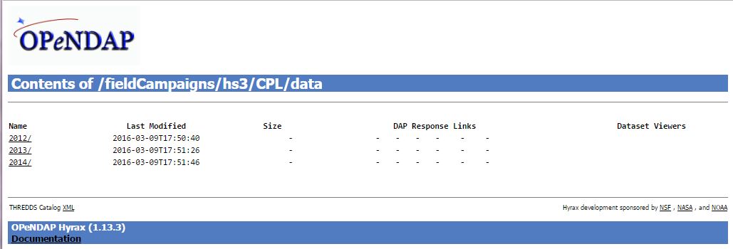
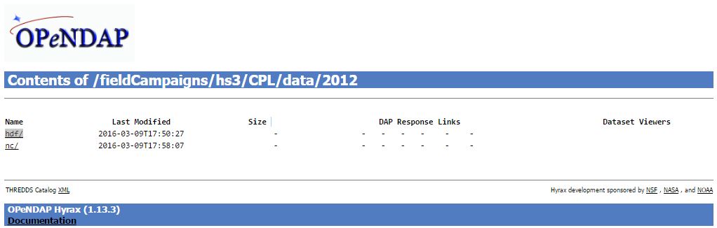
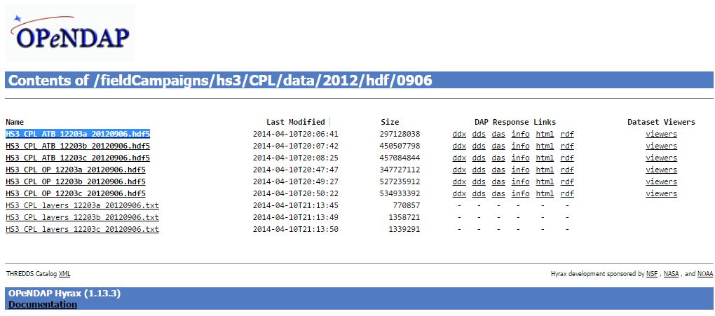
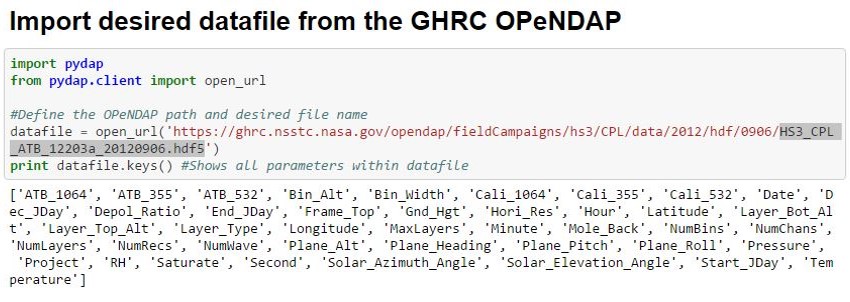
Within the Python script, to change the default data file to one you want to use, simply paste your file name to the "datafile" variable in the region highlighted below. Make sure to update the OPeNDAP URL path to reflect the year and day of the datefile.
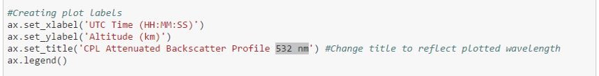
To create the data plot, simply run the script. A window will pop up containing the desired plot.
This data requires additional processing to quality control and remove erroneous data values. Please refer to the User Guide and PI Documentation for additional information on data quality.
If you would like the run this data recipe as an iPython Notebook, run externally through the Jupyter Notebook web application. More information on Jupyter can be found here.
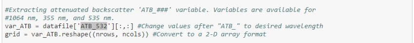
The Python script and iPython Notebook may be reused and altered to plot additional CPL data variables not used in this data recipe. Additional documentation is provided within the code to help walk you through the content.
| Dataset Name | Hurricane and Severe Storm Sentinel (HS3) Global Hawk Cloud Physics Lidar (CPL) |
| Platform | Global Hawk Unmanned Aerial Vehicle (UAV) |
| Instrument | Cloud Precipitation Lidar (CPL) |
| Science Parameter | Attenuated Total Backscatter |
| Format | HDF-EOS5 |
| Data Information |
|
| Variable | Description | Dimension | Units | Scale Factor |
|---|---|---|---|---|
| time | Time | n/a | seconds | none |
| bin_Alt | Altitude in km for each vertical bin | 1D | kilometer | none |
| Dec_JDay | Decimal day of year to 5 decimal places (second) for current profile | 1D | days since 2012-01-01T00:00:00Z | none |
| Date | Date for flight | 1D | text | none |
| ATB_1064 | Attenuated total backscatter collected for 1064 nm channel | 2D | km-1 sr-1 | none |
| ATB_355 | Attenuated total backscatter collected for 355 nm channel | 2D | km-1 sr-1 | none |
| ATB_532 | Attenuated total backscatter collected for 532 nm channel | 2D | km-1 sr-1 | none |

Dec 1st, 2022