ISS LIS Lightning Flash Location Quickview using Python 3.0 and GIS
The Lightning Imaging Sensor (LIS) onboard the International Space Station (ISS) retrieves optical lightning measurements over the majority of the Earth. This data recipe guides the user through a Python script that enables visualization of ISS LIS lightning flash locations. It is designed to compile information from a series of user-selected ISS LIS swath data files and generate a gridded heat map plot of lightning flash locations. In addition, a CSV file is generated containing the lightning flash coordinates in a format that can be input into other software. For this data recipe, the CSV file will be used to plot lightning flash locations in ESRI’s ArcMap GIS software.
| Data Recipe Type | |
|---|---|
| Visualization | |
| TYPE | ACCESS | ||
|---|---|---|---|
|
| Python 3 Script |
| ArcMap 10.2+ |
This data recipe uses the ISS LIS Science Data, however, this routine may be applied to the other ISS LIS data products offered by GHRC. More information and additional resources about this particular dataset can be accessed here.
This data recipe is available as a Python script. To run the script, please install the following Python packages: numpy, matplotlib, cartopy, netCDF4, and csv. The pre-installed Python sys, os, and glob packages will also be used. Additional information on installing Python packages is available here.
Follow this link to the GHRC DAAC Data-Recipe GitHub folder and obtain the ISS LIS Lightning Flash Location Quickview Python script titled “ISS_LIS_FlashLoc_Quickview_Python3.py”.
You can preview the script by clicking the file name. To download the script, click the “Download” button located in the top right corner of the window. Save the file to a desired folder location on your computer.
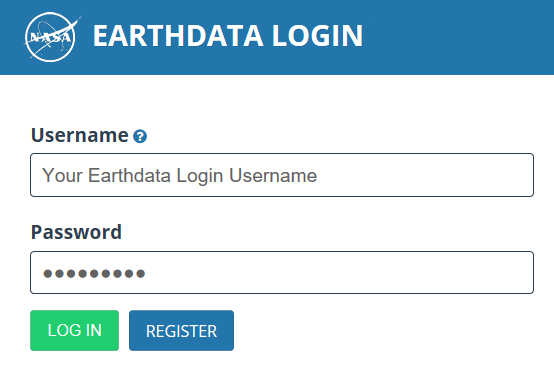
To download the data needed for this data recipe, a free NASA Earthdata user account is required. If you do not have an account, you will first need to create one by clicking the “Register” button (shown below) and following the required steps.
Once your NASA Earthdata account has been created, you can download the ISS LIS netCDF-4 data files directly here (you may have to re-enter Earthdata account information if not already logged in). Follow the link to select and download the data files of your choice. Save these files to a desired location on your computer.
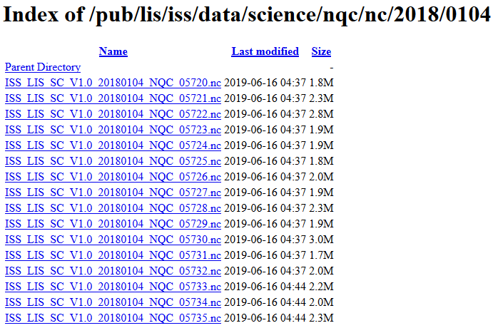
For this data recipe, we focus on January 4, 2018 because the data captured lightning from the bombogenesis winter weather event along the U.S. East coast. Since ISS LIS data files represent individual swaths collected within a day, all data files generated for January 4th were downloaded for this data recipe (shown in the image below). The Python code can handle plotting anywhere from one data file to many data files covering a time period of your choosing.
There are two ways to run the Python script: from the Python Prompt window or from the console of your Python environment.To simply run the script from the Python Prompt, open your Python environment’s prompt window. Make sure the required Python packages outlined in the “How to Use” section are installed and check that your current directory is the location where the ISS_LIS_FlashLoc_Quickview_Python3.py script is saved. The following two arguments will be passed in the command line. After initiating Python by typing “python”, add a space and paste the name of the script: ISS_LIS_FlashLoc_Quickview_Python3.py. Add a space and then enter the path to the directory holding the ISS LIS files you downloaded. An example of the command line statement is shown below:
(base) C:\Users\name > python ISS_LIS_FlashLoc_Quickview_Python3.py D:\data_recipes\iss_lis\data
After pressing enter, you will find both a CSV file containing the lightning flash location coordinates and a PNG heat map image inside the same folder that holds the ISS LIS data files. Examples of these files are shown later in this data recipe.
If you would like to run the script inside your Python console, the following steps will guide you through each step in the script to plot the lightning locations and generate the CSV file.
Open the Python environment installed on your computer and as previously noted, make sure the required Python packages outlined in the “How to Use” section are installed.
Navigate to the location on your computer where the ISS_LIS_FlashLoc_Quickview_Python3.py file is saved and open the file within your Python environment. You may also directly copy the script text from the GitHub script preview and paste it into a blank Python file within your Python environment.
At the very beginning of the script file is a header that describes the script’s function. Below the header is where the code begins. First, all of the required packages and subpackages are imported (shown below). Below the import section, an initial file path is defined that will be passed into the main( ) function. (It can be changed by passing a different file path as an argument to the main( ) function in the Python console when running the script; this is addressed in Step 15). Navigate to the folder on your computer where you saved the ISS LIS netCDF-4 data files. From the address bar, copy the file path and paste it inside the quotations behind the “file_path” variable. An example path is included in the script and shown in green text in the image below.

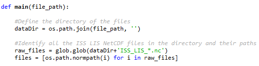
The next section of code is where the main( ) function begins. This section defines the data directory and identifies only the ISS LIS files within the directory. It also loops through each ISS LIS file path to ensure they are formatted correctly. The image below shows the code section that performs these tasks.
The ISS LIS netCDF-4 data files contain many different variables describing each lightning observation. For this data recipe we will use the “lightning_flash_lat”, “lightning_flash_lon”, “orbit_summary_TAI93_start”, and “orbit_summary_TAI93_end” variables.

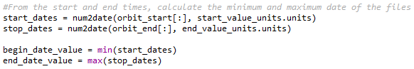
Once the start and end times are collected into their respective lists, the units are converted into the date and UTC time. Lastly, the start and end dates are identified by finding the maximum and minimum dates.
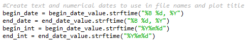
This section creates the text for the start and end dates using the dates calculated in Step 7. These will be used when naming files and adding the title to the plot image.
This Python script generates a CSV file of lightning flash location coordinates that can be used within other software. First, the CSV file name and path are designated. For the variable “csvfile”, the script will save the CSV file in the same directory that holds the ISS LIS netCDF-4 data files, specified at the beginning of the script. This section creates the CSV file name using the dates from Step 8.
![]()
It is now time to extract the lightning flash locations. The “lightning_flash_lat” and “lightning_flash_lon” variables contain the latitude and longitude coordinates of ISS LIS detected lightning flash locations. This script goes to the file directory where the ISS LIS data files are stored, loops through each file and pulls out the latitude and longitude flash location coordinates. These values are added onto two arrays (flash_lat and flash_lon) so that all lightning flash locations are collected within one location, not spread across several files.
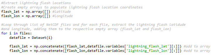
Note: If you would like to augment the code and extract other variables, you can change the data variables shown in green text above. The other variables available within the ISS LIS netCDF-4 data files are listed in the ISS LIS datasets user guide.
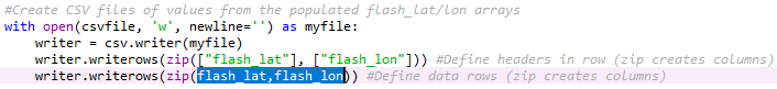
Once these values are extracted, the next portion of the code generates the CSV file. If you do not want to generate a CSV file, simply comment out this portion of the code by inserting a "#" symbol at the beginning of each line, as shown below.
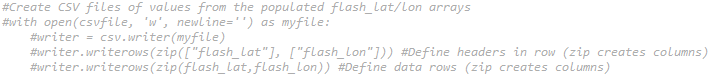
To change the header names of the columns, change the text highlighted in blue below to a header name of your choosing.

This section of the code formats a hex grid heat map plot of flash locations using the hexagonal binning plot, or "hexbin" function. This function creates a hex grid, a grid with hexagon shaped cells, over the map domain and identifies all of the lighting flashes that occur within each cell. The user can change the size of the hex grid cells by adjusting the "gridsize" variable highlighted below. The "gridsize" is the number of hexagons in the x-direction. In this example, "gridsize=300" means that there are 300 hexagons in the x-direction. The number of cells in the y-direction is adjusted so that all hexagons in the grid are uniform. If you would like to define the number of cells in both the x- and y-direction, you can input two elements as (x, y) for the "gridsize". In the final plot, each hex grid cell represents a total count of flashes occurring within a specific “area” or bin size. You can change how the color map is applied to each hexagon in the plot by changing the "bins" variable (in the last line of code below). The types of scales and values that can be assigned to "bins" are detailed here. In this example, "bins" is set to "log" to assign the hexagon colors using a logarithmic scale; making the behavior of the data more visible to the viewer. This "log" scale will also be reflected in the labels applied to the colorbar created in Step 13.

This section creates the map features for the plot background, formats the plot labels, and creates the color scale bar for the lightning bins. You can change the extent of the plot by changing the latitude and longitude coordinates defined for the map extent feature highlighted below. The format for the coordinates is [°W, °E, °S, °N].

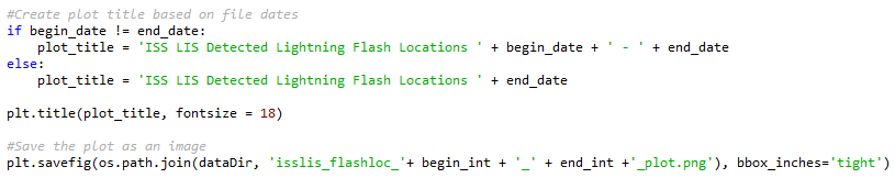
If the ISS LIS files you are creating a plot for cover multiple dates, that date range will need to be noted in the plot title. This section specifies the plot title based on the dates of the files. If there are multiple dates, the title will include the begin and end dates. However, if the ISS LIS files cover just one date, the title will only include that single date. Lastly, the plot is saved to the directory containing the data files.
Run the script from your Python console. This will generate the plot image and CSV file. You can change the directory from which the ISS LIS files are pulled by entering the path (in quotations) into the main( ) function and pressing enter within the console. An example is shown below:
![]()
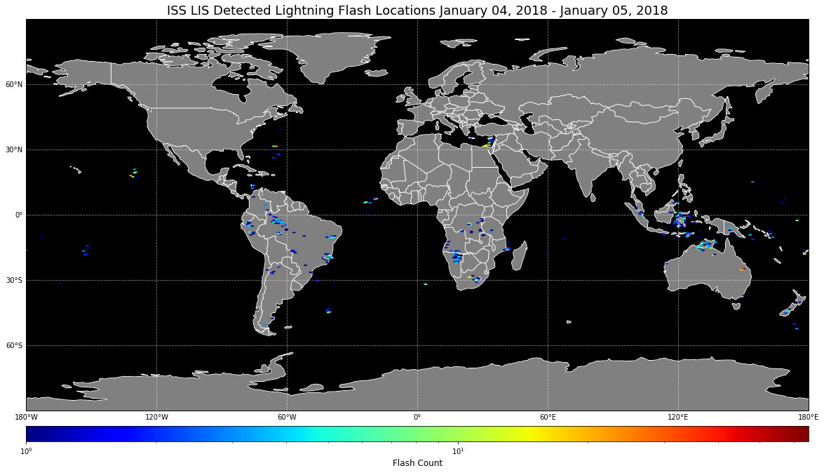
The plot image will appear in the console and be saved as a PNG image file to the folder where the data files are located. The plot will be named in the following format: isslis_flashloc_[begin date]_[end date]_plot.png. It should look similar to the image below.
(Note: [begin date] and [end date] are formatted: yyyymmdd where yyyy = four-digit year, mm = two-digit month, and dd = two-digit day)
The CSV file will also be saved to the directory containing the ISS LIS data files and is named in the following format: isslis_flashloc_[begin date]_[end date].csv. Navigate to this location on your computer and open the CSV file. In Excel, the CSV file should look similar to the image below.

This file may be used to plot the flash locations in other software. For this data recipe we will demonstrate plotting it in ESRI’s ArcMap. Close the CSV file.
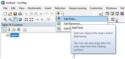
Open your ArcMap Desktop application. For this tutorial, ArcMap 10.2 was used. Click the “Add Data” button to add the CSV file as shown.

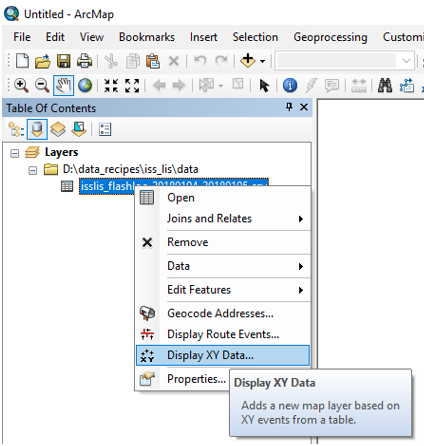
To plot the coordinates in the file, right click the flash location table layer and select “Display XY Data”.
A “Display XY Data” window will open. The “X Field” and “Y Field” should auto populate. Double check the fields and use the drop down arrows to set the “X Field” to “flash_lon” and the “Y Field” to “flash_lat”. Then click “OK” to plot.


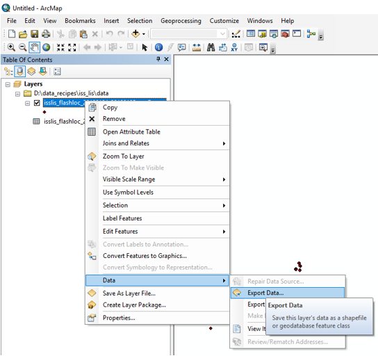
To save the flash locations as a shapefile, right click on the flash location data layer then select “Export Data” and save the file to a desired location.
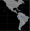
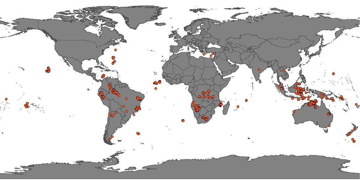
The ISS LIS lighting flash locations should plot similar to the map below when combined with a global shapefile. You may then use these points for other types of analysis and map making.
This Python script may be reused and altered as needed to plot additional data variables not used in this example.
The GHRC ISS LIS data products in netCDF-4 format may be used with this data recipe.
| Dataset Name | Non-Quality Controlled Lightning Imaging Sensor (LIS) on the International Space Station (ISS) Science Data |
| Platform | The International Space Station (ISS) |
| Instrument | Lightning Imaging Sensor (LIS) |
| Science Parameter | Lightning flash location |
| Format | netCDF-4 |
| Data Information |
|
| Variable | Description | Dimension | Units | Scale Factor |
|---|---|---|---|---|
| lightning_flash_lat | Latitude coordinate of lightning flash | 1D | degrees | none |
| lightning_flash_lon | Longitude coordinate of lightning flash | 1D | degrees | none |

Dec 2nd, 2022