OTD Lightning Flash Location Quickview using Python 3.0 and GIS
The Optical Transient Detector (OTD) was a space-based lightning detection instrument that retrieved optical lightning measurements over Earth between +/- 75 degrees latitude. It operated from 1995 to 2000 as a prototype for the Lightning Imaging Sensor (LIS). This data recipe guides the user through a Python script that enables visualization of OTD lightning flash locations. It is designed to compile information from a series of user-selected OTD data files and generate a gridded heat map plot of lightning flash locations. In addition, a CSV file is generated containing the lightning flash coordinates in a format that can be input into other software. For this data recipe, the CSV file will be used to plot lightning flash locations in ESRI’s ArcMap GIS software.
| Data Recipe Type | |
|---|---|
| Visualization | |
| TYPE | ACCESS | ||
|---|---|---|---|
|
| Python 3 Script |
| ArcMap 10.2+ |
This data recipe uses the Optical Transient Detector (OTD) Lightning dataset. More information and additional resources for this dataset can be accessed here.
This data recipe is available as a Python script. To run the script, please install the following Python packages: numpy, matplotlib, cartopy, and pyhdf. The Python sys, os, glob, subprocess, re, datetime, tarfile, and csv packages will also be used and should be pre-installed. Additional information on installing Python packages is available here.
For Windows Users: The OTD HDF4 files are compressed and therefore require the 7-Zip archive software to extract the files. Make sure that 7-Zip is installed on your computer. The 7-Zip software can be downloaded here.
For Linux Users: If you are running Linux from a Windows system, you may have to install an X-Windows application in order to view graphics, for example Xming.
This Python script is available for both Windows and Linux operating systems. Follow this link to the GHRC DAAC Data-Recipes GitLab folder and obtain the OTD Lightning Flash Location Quickview Python script named “OTD_FlashLoc_Quickview.py” for Windows users and “OTD_FlashLoc_Quickview_Linux.py” for Linux users.
You can preview the script by clicking the file name. To download the script, click the “Download” button located in the top right corner of the window. Save the file to a desired location on your computer.
To download the data needed for this data recipe, a free NASA Earthdata user account is required. If you do not have an account, you will first need to create one by clicking the “Register” button (shown below) and following the required steps.

Note: The OTD data files are named using the Julian day instead of the month and day (shown below).

There are two ways to run this Python script: from your computer’s command line or from your Python console. To simply run the script from the command line, first open your computer’s prompt window and check that your current directory is the location where the OTD_FlashLoc_Quickview.py (OTD_FlashLoc_Quickview_Linux.py) script is saved. Make sure the required Python packages outlined in the “How to Use” section are installed. The following arguments will be passed in the command line. After initiating Python by typing “python”, add a space and paste the name of the script: OTD_FlashLoc_Quickview.py (OTD_FlashLoc_Quickview_Linux.py). Add a space and then enter the path to the directory holding the OTD files you downloaded. An example of the command line statement is shown below:
Windows
C:\Users\name > python OTD_FlashLoc_Quickview.py D:\data_recipes\otd\
Linux
$ python OTD_FlashLoc_Quickview_Linux.py /home/user/data_recipes/otd/
After pressing enter, you will now find a CSV file containing the lightning flash location coordinates and a PNG heat map image inside the directory you specified. Examples of these files are shown later in this data recipe.
If you would like to run the script inside your Python console, the following steps will guide you through each step in the script to plot the lightning locations and generate a CSV file containing the coordinates for each lightning flash location.
Open the Python environment installed on your computer and as previously noted, make sure the required Python packages outlined in the “How to Use” section are installed.
Navigate to the location on your computer where the OTD_FlashLoc_Quickview.py (OTD_FlashLoc_Quickview_Linux.py) file is saved and open the file within your Python environment. You may also directly copy the script text from the GitLab script preview and paste it into a blank Python file within your Python environment.
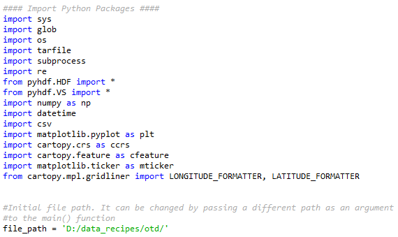
At the very beginning of the script file is a header that describes the script’s function. Below the header is where the code begins. First, all of the required packages and subpackages are imported (shown below). Below the import section, an initial file path is defined that will be passed into the main( ) function. (It can be changed by passing a different file path as an argument to the main( ) function in the Python console when running the script; this is addressed in Step 20. Navigate to the location on your computer where you saved the OTD HDF4 TAR data files. From the address bar, copy the file path and paste it inside the quotations behind the “file_path” variable. An example path is included in the script and shown in green text in the image below.
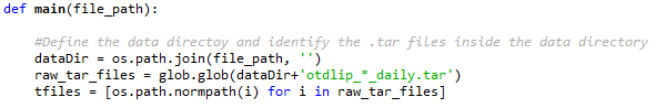
The next section of code is where the main( ) function begins. This section defines the data directory and identifies only the OTD TAR files within the directory. It also loops through each OTD file path to ensure they are formatted correctly. The image below shows the code section that performs these tasks.
In order to appropriately name the folders that will be created later in the script, the dates of the downloaded TAR files will need to be extracted from the file names. This section creates an empty list, loops through each TAR file in the directory, extracts the date from each file name, and adds each date to the initially empty list that was created earlier. Next, the minimum and maximum dates are identified so that the date range of the files can be used for directory and file naming.

This section creates a new directory to hold the untarred daily OTD files. The directory is named using the date range pulled from the TAR files in the previous step.

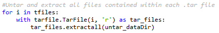
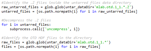
The OTD HDF4 files are compressed into daily TAR files. These files must be decompressed in order to view the OTD data variables. This section loops through each TAR file and extracts all of the files it contains. The files extracted from the TAR files are still compressed within a .Z file which we will decompress in the next step.
In this section, all of the .Z files are identified and decompressed.
First, the .Z files and their paths are identified. The 7-Zip software installed on your computer is used to extract the OTD HDF4 files from the .Z files (see the “How to Use” section for 7-Zip download information). The path assigned to the “z_location” variable is the standard location of the 7z.exe program file on most computer systems, however, check that your 7z.exe file is in this location. If it is not, make sure to change this variable to the correct path for your computer’s 7z.exe file. The second block of code loops through each .Z file and uses 7-Zip to extract the HDF4 files and place them in the target directory. The .Z files are deleted after extraction and the path to each HDF4 file is identified.

For Linux:
First, the .Z files and their paths are identified. Then the “uncompress” command is used to decompress the .Z files and reveal the OTD HDF4 files. Lastly, the path to each of these HDF4 files is identified.
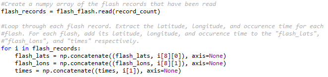
Here, empty Numpy arrays are created to hold the lightning flash latitude, longitude, and occurrence time values once they are extracted from the OTD HDF4 files.
![]()
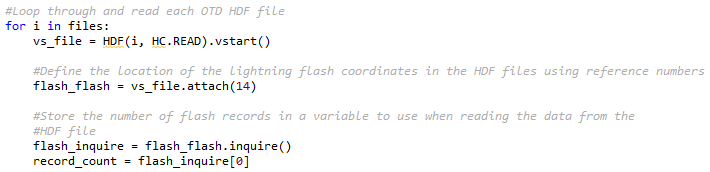
The OTD HDF4 data files contain multiple variables describing each lightning observation. For this data recipe we will use the “cent” and “TAI93” variables from the OTD HDF4 files, which describe the latitude and longitude of each flash, and the flash occurrence time in units of “seconds since 1993-01-01 00:00:00.000”. In Hierarchical Data Format (HDF) files, data are organized into groups and subgroups. In this section of code, the “pyhdf” package is used to read the HDF4 files. Reference numbers are used to identify the “Flash” group and subgroup containing data for individual lightning flashes. Next, the number of records in the file are identified so that this value can be used to read each record in the next step.
Now that the location of the lightning flash variables has been identified, this section can read each flash record contained in the file and for each of these records, extract the lightning flash latitude, longitude, and occurrence time. These extracted coordinates and times are then added to the empty arrays that were created in Step 11. This process is repeated for each HDF4 file.
This section handles the occurrence times of each lightning flash. First, the flash start and end times are identified from the array of times extracted from the HDF4 files in the previous step. Next, the “datetime” module is used to convert the times listed in the HDF4 files (“seconds since 1993-01-01 00:00:00.000”) to the standard UTC date and time. Lastly, these dates and times are converted to numerical and text strings so that they can be used in file names and in the title of the flash heat map.

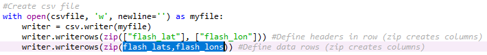
This Python script generates a CSV file containing lightning flash coordinates that can be used within other software. First, the CSV file name and path are designated. For the variable “csvfile”, the script will save this file in the original directory indicated at the beginning of the script. This section also creates the CSV file name using the dates from the previous step.

The next portion of the code generates the CSV file. If you do not want to generate a CSV file, simply comment out this portion of the code by inserting a ‘#’ symbol at the beginning of each line, as shown below.

To change the header names of the columns, change the text highlighted in blue below to the names of your choosing.
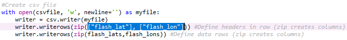
The next line of code defines what data variables will be included in the CSV file. For this example we use the "flash_lats" and "flash_lons" arrays containing the extracted flash location coordinates from Step 13.
This section of the code formats a hex grid heat map plot of flash locations using the hexagonal binning plot, or "hexbin" function. This function creates a hex grid, a grid with hexagon shaped cells, over the map domain and identifies all of the lighting flashes that occur within each cell. The user can change the size of the hex grid cells by adjusting the "gridsize" variable highlighted below. The "gridsize" is the number of hexagons in the x-direction. In this example, "gridsize=300" means that there are 300 hexagons in the x-direction. The number of cells in the y-direction is adjusted so that all hexagons in the grid are uniform. If you would like to define the number of cells in both the x- and y-direction, you can input two elements as (x, y) for the "gridsize". In the final plot, each hex grid cell represents a total count of flashes occurring within a specific “area” or bin size. You can change how the color map is applied to each hexagon in the plot by changing the "bins" variable (in the last line of code below). The types of scales and values that can be assigned to "bins" are detailed here. In this example, "bins" is set to "log" to assign the hexagon colors using a logarithmic scale; making the behavior of the data more visible to the viewer. This "log" scale will also be reflected in the labels applied to the colorbar that will be created in the next step.

This section creates the map features for the plot background, formats the plot labels, and creates the color scale bar for the lightning bins. You can change the extent of the plot by changing the latitude and longitude coordinates defined for the map extent feature highlighted below. The format for the coordinates is [°W, °E, °S, °N].

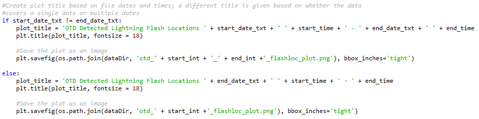
If you are creating a plot for multiple dates, that date range will need to be noted in the plot title. This section specifies the plot title based on he date/time of the files. If there are multiple dates/times, the title will include the begin and end dates/times. However, if just one OTD data file is plotted, the title will only include that single date with the range of times. Lastly, the plot is saved to the directory specified at the beginning of the script.
Run the script from your Python console. This will generate the plot image and CSV file. You can change the directory from which the OTD files are pulled by entering the path (in quotations) into the main( ) function and pressing enter within the console. An example is shown below:
![]()
The plot image will appear in the console and be saved as a PNG image file to the directory you specified. The plot image file will be named in the following format: otd_[begin date]_[end date]_flashloc_plot.png (or otd_[date]_flashloc_plot.png). It should look similar to the image shown below.
(Note: the dates in the plot filename are formatted: yyyymmdd where yyyy = four-digit year, mm = two-digit month, and dd = two-digit day)

The CSV file is also saved to the directory you specified and is named in the following format: otd_[begin date]_[end date]_flashloc.csv (or otd_[date]_flashloc.csv). Navigate to this location on your computer and open the CSV file. In Excel, the CSV file should look similar to the image below.

This file may be used to plot the flash locations in other software. For this data recipe, we will demonstrate plotting the flash locations in ESRI’s ArcMap. Close the CSV file.
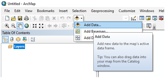
Open your ArcMap Desktop application. For this tutorial, ArcMap 10.2 was used. Click the “Add Data” button to add the CSV file as shown.
Navigate to the location on your computer where the CSV file is stored. You may have to create a new folder connection by clicking the “Connect to Folder” button near the top right corner of the “Add Data” window. Once in the correct location, double click the CSV file to add it as a table layer.

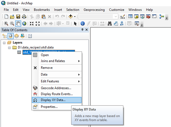
To plot the coordinates in the file, right click the flash location table layer and select “Display XY Data”.
A “Display XY Data” window will open. The “X Field” and “Y Field” should auto populate. Double check the fields and use the drop down arrows to set the “X Field” to “flash_lon” and the “Y Field” to “flash_lat”. Then click “OK” to plot.

A window will pop up that reads “Table Does Not Have Object-ID Field”. Click “OK”.

The lightning flash points should display in the ArcMap window.
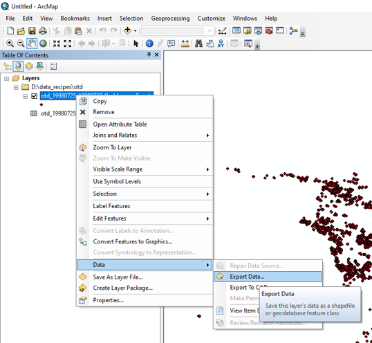
To save the flash locations as a shapefile, right click on the flash location data layer then select “Export Data” and save the file to a desired location.
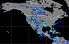
The OTD lighting flash locations should plot similar to the map below when combined with a global shapefile. You may then use these points for other types of analysis and map making.

This Python script may be reused and altered as needed to plot additional data variables not used in this example.
The GHRC OTD Lightning Data in HDF4 format may be used with this data recipe.
| Dataset Name | Optical Transient Detector (OTD) Lightning |
| Platform | OrbView-1 (formerly MicroLab-1) |
| Instrument | Optical Transient Detector (OTD) |
| Science Parameter | Lightning flash location |
| Format | HDF4 |
| Data Information |
|
| Variable | Description | Dimension | Units | Scale Factor |
|---|---|---|---|---|
| Flash/flash.cent | Latitude and longitude coordinates of lightning flash | - | degrees | none |

Dec 2nd, 2022